Returns the item correlation matrix (and when K dimensions have been specified, K matrices) that the function mdepriv internally generates
when the argument
method="bv"and the argumentbv_corr_type="mixed"or"pearson"or when the argument
wais specified and the argumentwb="mixed"or"pearson".
Permits inspection of the correlation structure and can be used for complementary analytic purposes such as factor analysis or biplots.
Arguments
- data
a
data.frameor amatrixwith columns containing variables representing deprivation items measured on the [0,1] range. Optionally a column with user defined sampling weights (s. argumentsampling_weights) can be included.- items
a character string vector or list of such vectors specifying the indicators / items within the argument
datafrom which the deprivation scores are derived. If the user inputs a list with more than one vector, the items are grouped in dimensions. By naming the list elements, the user defines the dimensions' names. Else, dimensions are named by default"Dimension 1"to"Dimension K"where K is the number of dimensions.- sampling_weights
a character string corresponding to column heading of a numeric variable within the argument
datawhich is specified as sampling weights. By default set toNA, which means no specification of sampling weights.- corr_type
a character string selecting the correlation type. Available choices are
"mixed"(default) and"pearson". The option"mixed"detects automatically the appropriate correlation type"pearson","polyserial"or"polychoric"for each pair of items (s. Details).- output
a character string vector selecting the output. Available choices are
"numeric"(default),"type"or"both"."numeric"delivers a numeric correlation matrix or list of such matrices. (the latter if theitemsare grouped in more than one dimension)."type"delivers the correlation type applied to each pair of items in a matrix, respectively list of matrices analog to the numeric output."both"combines the"numeric"and"type"as a list.
Value
Either a single matrix or a list composed of several matrixes (s. argument "output").
Details
The calculation of the correlation coefficient for a pair of items is based on the function weightedCorr.
When setting the argument corr_type to "mixed"
the appropriate correlation type "pearson", "polyserial" or "polychoric"
is automatically detected for each pair of items by the following rules:
"pearson": both items have > 10 distinct values."polyserial": one item has \(\le\) 10, the other > 10 distinct values."polychoric": both items have \(\le\) 10 distinct values.
When the argument corr_type is set to "pearson" this correlation type is forced on all item pairs.
Depending on the correlation type(s) used, the matrix may not be positive semidefinite and therefore not immediately suitable for purposes such as factor analysis.
This is more likely to happen when some of the items are binary.
The function nearPD will produce the nearest positive definite matrix.
Examples
head(simul_data, 3) # data used for demonstration
#> id y1 y2 y3 y4 y5 y6 y7 sampl_weights
#> 1 1 0 0 0 0.0 0.369 0.174 0.196 0.556
#> 2 2 1 0 1 0.2 0.762 0.832 1.000 1.500
#> 3 3 0 1 1 0.4 0.708 0.775 0.833 0.973
corr_mat(simul_data, c("y1", "y4", "y5", "y6")) # default output: numeric
#> y1 y4 y5 y6
#> y1 1.0000000 0.81597841 0.8574640 0.32881030
#> y4 0.8159784 1.00000000 0.8083585 0.05629782
#> y5 0.8574640 0.80835852 1.0000000 -0.10943492
#> y6 0.3288103 0.05629782 -0.1094349 1.00000000
corr_mat(simul_data, c("y1", "y4", "y5", "y6"), output = "type")
#> y1 y4 y5 y6
#> y1 "polychoric" "polychoric" "polyserial" "polyserial"
#> y4 "polychoric" "polychoric" "polyserial" "polyserial"
#> y5 "polyserial" "polyserial" "pearson" "pearson"
#> y6 "polyserial" "polyserial" "pearson" "pearson"
corr_mat(simul_data, c("y1", "y4", "y5", "y6"), output = "both")
#> $numeric
#> y1 y4 y5 y6
#> y1 1.0000000 0.81597841 0.8574640 0.32881030
#> y4 0.8159784 1.00000000 0.8083585 0.05629782
#> y5 0.8574640 0.80835852 1.0000000 -0.10943492
#> y6 0.3288103 0.05629782 -0.1094349 1.00000000
#>
#> $type
#> y1 y4 y5 y6
#> y1 "polychoric" "polychoric" "polyserial" "polyserial"
#> y4 "polychoric" "polychoric" "polyserial" "polyserial"
#> y5 "polyserial" "polyserial" "pearson" "pearson"
#> y6 "polyserial" "polyserial" "pearson" "pearson"
#>
# with sampling weights (3rd argument)
corr_mat(simul_data, c("y1", "y4", "y5", "y6"), "sampl_weights")
#> y1 y4 y5 y6
#> y1 1.0000000 0.79871297 0.84893375 0.37055782
#> y4 0.7987130 1.00000000 0.81370895 0.04023532
#> y5 0.8489338 0.81370895 1.00000000 -0.09680152
#> y6 0.3705578 0.04023532 -0.09680152 1.00000000
# choose correlation type
corr_mat_default <- corr_mat(simul_data, c("y1", "y4", "y5", "y6"))
corr_mat_mixed <- corr_mat(simul_data, c("y1", "y4", "y5", "y6"), corr_type = "mixed")
all.equal(corr_mat_default, corr_mat_mixed) # "mixed is corr_type's default
#> [1] TRUE
# force a correlation type on all pairs of items
corr_mat(simul_data, c("y1", "y4", "y5", "y6"), corr_type = "pearson")
#> y1 y4 y5 y6
#> y1 1.0000000 0.60056932 0.4629204 0.21372370
#> y4 0.6005693 1.00000000 0.6792278 0.07185579
#> y5 0.4629204 0.67922776 1.0000000 -0.10943492
#> y6 0.2137237 0.07185579 -0.1094349 1.00000000
# grouping items in dimensions
corr_mat(simul_data, list(c("y1", "y4", "y5", "y6"), c("y2", "y3", "y7")))
#> $`Dimension 1`
#> y1 y4 y5 y6
#> y1 1.0000000 0.81597841 0.8574640 0.32881030
#> y4 0.8159784 1.00000000 0.8083585 0.05629782
#> y5 0.8574640 0.80835852 1.0000000 -0.10943492
#> y6 0.3288103 0.05629782 -0.1094349 1.00000000
#>
#> $`Dimension 2`
#> y2 y3 y7
#> y2 1.00000000 0.064950690 0.060486856
#> y3 0.06495069 1.000000000 0.001620888
#> y7 0.06048686 0.001620888 1.000000000
#>
# customized group / dimension labels
corr_mat(simul_data, list("Group A" = c("y1", "y4", "y5", "y6"),
"Group B" = c("y2", "y3", "y7")))
#> $`Group A`
#> y1 y4 y5 y6
#> y1 1.0000000 0.81597841 0.8574640 0.32881030
#> y4 0.8159784 1.00000000 0.8083585 0.05629782
#> y5 0.8574640 0.80835852 1.0000000 -0.10943492
#> y6 0.3288103 0.05629782 -0.1094349 1.00000000
#>
#> $`Group B`
#> y2 y3 y7
#> y2 1.00000000 0.064950690 0.060486856
#> y3 0.06495069 1.000000000 0.001620888
#> y7 0.06048686 0.001620888 1.000000000
#>
# mdepriv output / returns as template for corr_mat arguments
# items grouped as dimensions
dim <- list("Group X" = c("y1", "y4", "y5", "y6"), "Group Z" = c("y2", "y3", "y7"))
# model: betti-verma ("bv"): correlation type = pearson, rhoH = NA (data driven)
bv_pearson <- mdepriv(simul_data, dim, "sampl_weights",
method = "bv", bv_corr_type = "pearson", output = "all")
# use model output as arguments
corr_mat(bv_pearson$data, bv_pearson$items, bv_pearson$sampling_weights,
corr_type = bv_pearson$wb, output = "both")
#> $numeric
#> $numeric$`Group X`
#> y1 y4 y5 y6
#> y1 1.0000000 0.58315592 0.45257771 0.23819918
#> y4 0.5831559 1.00000000 0.68561919 0.05063697
#> y5 0.4525777 0.68561919 1.00000000 -0.09680152
#> y6 0.2381992 0.05063697 -0.09680152 1.00000000
#>
#> $numeric$`Group Z`
#> y2 y3 y7
#> y2 1.00000000 0.06293436 0.03891441
#> y3 0.06293436 1.00000000 0.01315840
#> y7 0.03891441 0.01315840 1.00000000
#>
#>
#> $type
#> $type$`Group X`
#> y1 y4 y5 y6
#> y1 "pearson" "pearson" "pearson" "pearson"
#> y4 "pearson" "pearson" "pearson" "pearson"
#> y5 "pearson" "pearson" "pearson" "pearson"
#> y6 "pearson" "pearson" "pearson" "pearson"
#>
#> $type$`Group Z`
#> y2 y3 y7
#> y2 "pearson" "pearson" "pearson"
#> y3 "pearson" "pearson" "pearson"
#> y7 "pearson" "pearson" "pearson"
#>
#>
# model: user defined double weighting
# 1st factor = wa = "equal", 2nd factor = wa = "mixed" (correlation type),
# rhoH = NA (data driven)
eq_mixed <- mdepriv(simul_data, dim, "sampl_weights",
wa = "equal", wb = "mixed", output = "all")
# use model output as arguments
corr_mat(eq_mixed$data, eq_mixed$items, eq_mixed$sampling_weights,
corr_type = eq_mixed$wb, output = "both")
#> $numeric
#> $numeric$`Group X`
#> y1 y4 y5 y6
#> y1 1.0000000 0.79871297 0.84893375 0.37055782
#> y4 0.7987130 1.00000000 0.81370895 0.04023532
#> y5 0.8489338 0.81370895 1.00000000 -0.09680152
#> y6 0.3705578 0.04023532 -0.09680152 1.00000000
#>
#> $numeric$`Group Z`
#> y2 y3 y7
#> y2 1.00000000 0.10363632 0.05015889
#> y3 0.10363632 1.00000000 0.01656435
#> y7 0.05015889 0.01656435 1.00000000
#>
#>
#> $type
#> $type$`Group X`
#> y1 y4 y5 y6
#> y1 "polychoric" "polychoric" "polyserial" "polyserial"
#> y4 "polychoric" "polychoric" "polyserial" "polyserial"
#> y5 "polyserial" "polyserial" "pearson" "pearson"
#> y6 "polyserial" "polyserial" "pearson" "pearson"
#>
#> $type$`Group Z`
#> y2 y3 y7
#> y2 "polychoric" "polychoric" "polyserial"
#> y3 "polychoric" "polychoric" "polyserial"
#> y7 "polyserial" "polyserial" "pearson"
#>
#>
# model: user defined double weighting
# 1st factor = wa = "bv", 2nd factator = wb = "diagonal"
# (all off-diagonal correlations = 0), rhoH = NA (irrelvant)
bv_diagonal <- mdepriv(simul_data, dim, "sampl_weights",
wa = "bv", wb = "diagonal", output = "all")
# use model output as arguments
try(
corr_mat(bv_diagonal$data, bv_diagonal$items, bv_diagonal$sampling_weights,
corr_type = bv_diagonal$wb, output = "both")
)
#> Error in match.arg(corr_type) : 'arg' should be one of "mixed", "pearson"
# triggers an error because:
bv_diagonal$wb
#> [1] "diagonal"
# if corr_type is left as the default or set to a valid option, then ...
corr_mat(bv_diagonal$data, bv_diagonal$items, bv_diagonal$sampling_weights)
#> $`Group X`
#> y1 y4 y5 y6
#> y1 1.0000000 0.79871297 0.84893375 0.37055782
#> y4 0.7987130 1.00000000 0.81370895 0.04023532
#> y5 0.8489338 0.81370895 1.00000000 -0.09680152
#> y6 0.3705578 0.04023532 -0.09680152 1.00000000
#>
#> $`Group Z`
#> y2 y3 y7
#> y2 1.00000000 0.10363632 0.05015889
#> y3 0.10363632 1.00000000 0.01656435
#> y7 0.05015889 0.01656435 1.00000000
#>
# ... it works
# for the arguments data, items and sampling_weights the ...
# ... corresponding mdepriv outputs are always valid
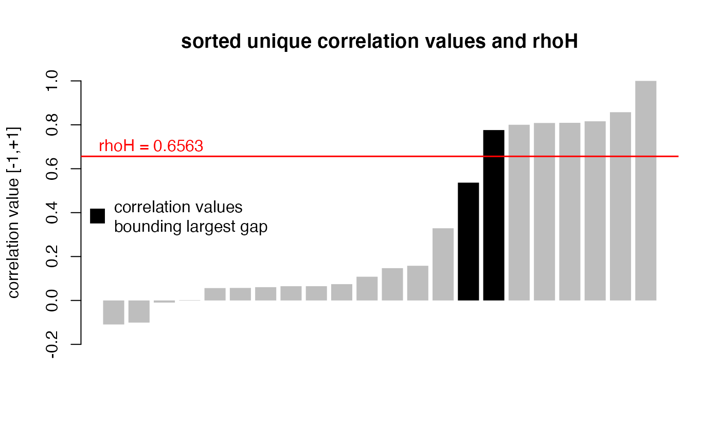
# plot unique correlation values and their relation to rhoH
items_sel <- c("y1", "y4", "y5", "y6", "y2", "y3", "y7") # a selection of items
corr_mat <- corr_mat(simul_data, items_sel) # corr_type default: "mixed"
rhoH <- mdepriv(simul_data, items_sel, method = "bv", output = "rhoH")
# bv_corr_type default: "mixed"
corr_val <- unique(sort(corr_mat)) # sorted unique correlation values
dist_rhoH_corr <- abs(corr_val - rhoH) # distance of corr. values to rhoH
bounding_rhoH <- abs(dist_rhoH_corr - min(dist_rhoH_corr)) < 10^-10
# TRUE if one of the two corr. values bounding rhoH else FALSE
corr_val_col <- ifelse(bounding_rhoH, "black", "gray") # colors for corr. values
barplot(corr_val,
col = corr_val_col,
border = NA,
ylim = c(-0.2, 1),
ylab = "correlation value [-1,+1]",
main = "sorted unique correlation values and rhoH"
)
abline(h = rhoH, col = "red", lwd = 1.5)
text(0, rhoH + 0.05, paste0("rhoH = ", round(rhoH, 4)), adj = 0, col = "red")
legend("left",
"correlation values\nbounding largest gap",
col = "black", pch = 15, pt.cex = 2, bty = "n"
)